Keyword [Compact Bilinear Pooling]
Gao Y, Beijbom O, Zhang N, et al. Compact bilinear pooling[C]//Proceedings of the IEEE Conference on Computer Vision and Pattern Recognition. 2016: 317-326.
1. Overview
此前提出的full bilinear模型存在一些问题(channel=512, k=1000时)
- 输出512512(260000)维度,导致后续的分类器参数很大(1000512*512≈250 million)
- storage expensive (2TB)
- 无法扩展到spatial pyramid matching、domain adaptation等
- 在few-shot learning上存在困难(如参数太多很容易过拟合)
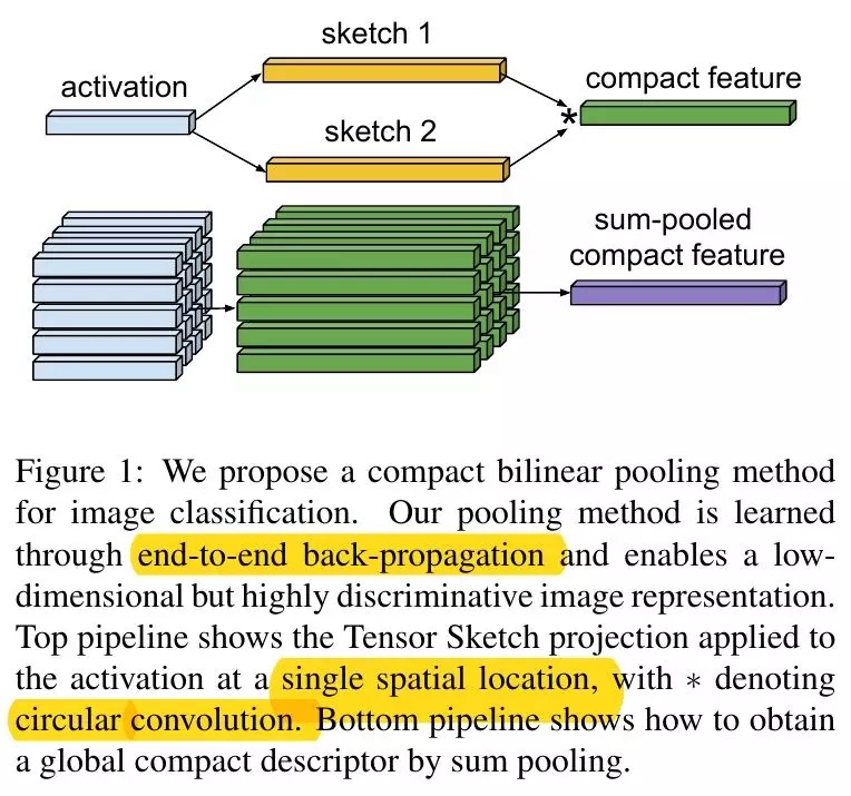
基于上述问题,论文提出两种compact bilinear pooling方法
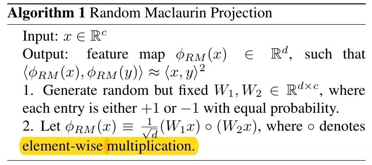
- Random Maclaurin Projection (RM)
- Tensor Sketch Projection (TS)
具有以下特点
- 减少两个数量级维度的同时,几乎不降低性能
- back-propagation efficient且end-to-end train

实际上,full bilinear方法在只使用2%特征维度情况下,与论文提出方法的性能相似。因此,98%的特征都是冗余的。
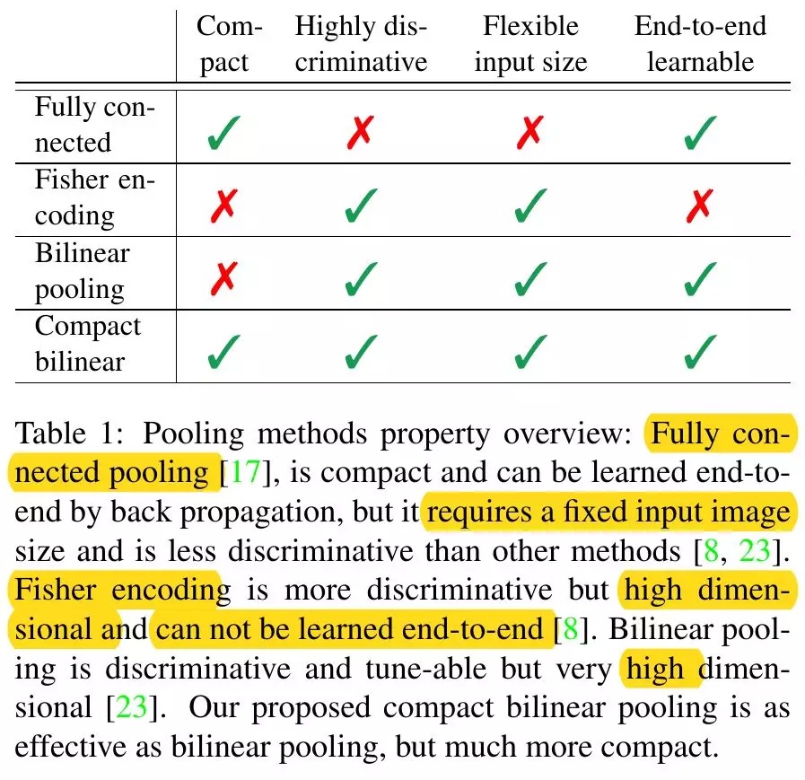
1.1. 与其他方法比较
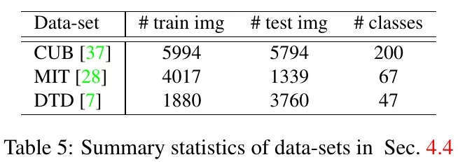
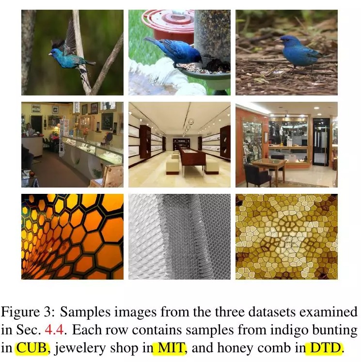
1.2. 数据集
- CUB(鸟类)
- MIT(室内场景)
- DTD(结构)
2. Pooling方法
2.1. circular convolution(循环卷积)
a=[1,2,3,4], b=[5,6,7,8], a*b计算过程
- a逆时针固定在圆上,b顺时针固定在圆上。对应相乘求和结果y(0)=66.
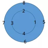
- a顺时针旋转一位,计算y(1)=68
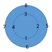
最终y的维度与a,b相同
2.2. Bilinear Sum Pooling
(h, w, c)->(h,w, cc)->(cc)
3. Compact Bilinear Models
3.1. Full Bilinear Pooling
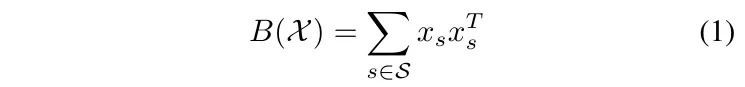
- S. set of location, 数量为height*width
- X. local descriptors, 输入特征图每个点的值(长度为channel数c)
维度变化(h, w, c)->(h, w, cc)->(cc)
3.2. Compact Bilinear Pooling
找到Φ(x)∈R^d使得 $Φ(x) ≈ xx^T$
- Random Maclaurin
- Tensor Sketch
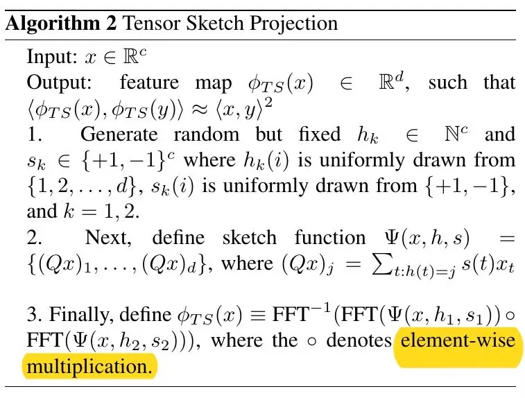

- stream_1, stream_2;(b, 512, h, w), d=8000
- 初始化h_1, s_1, h_2, s_2;(512),构造矩阵sparse_sketch_matrix1,sparse_sketch_matrix2;(512, 8000)
- reshape stream_1,stream_2;(bhw, 512)
- sketch=stream*sparse_sketch_matrix; (bhw, 8000)
- FFT(sketch_1)·FFT(sketch_2); (bhw, 8000)
- IFFT; (bhw, 8000)
- reshape (b, h, w, 8000)
- sum pooling; (b, 8000)
3.3. 计算时间

在Caffe K40c GPU下
- VGG16 forward backward时间为312ms
- Bilinear pooling 0.77ms
- TS(d=4096) 5.03ms,FFT计算量比矩阵运算大
4. Experiments
4.1. Pooling Methods
- Full Bilinear Pooling
- Compact Bilinear Pooling. 相对于512*512(≈260000)特征维度,8000维度足够表示特征。fine tuning能够提高效果,但提升很小。
- Fully Connected Pooling
- Improved Fisher Encoding. 对输出进行64 GMM编码
4.2. 维数&方式比较
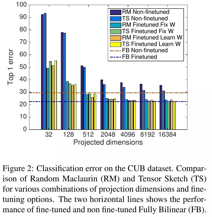
- 在维度很小时,fine tune能够显著提升效果
- 维度在2000~8000合适
4.3. 与PCA比较
PCA Bilinear通过在bilinear layer前插入1*1Conv实现,初始化为PCA权重。

4.4. 实验结果

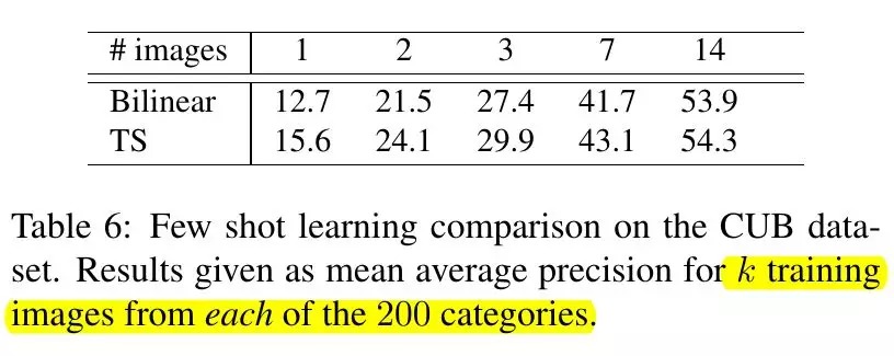
4.5. Few Shot Learning
- 训练样本数量与分类器假设空间(hypothesis space)大小相关
- 实验证明低维度表示更适合few-shot learning